Because it’s fast, fun, and wildly creative. You go from idea to game in seconds. Great for prototyping, learning, or impressing your friends at brunch.
Imagine typing “a Flappy Bird clone” and watching it pop open in your browser — ready to play. No design. No dev work. Just vibes and velocity.
Don’t just eval. That’s dangerous. ast.literal_eval is safer and stricter.
Step 5 — Generate the game code using your prompt
def create_game_code(game_name: str) -> str:
   prompt = f”””
   You are a game developer.
   You are given a game name.
   Create code for that game in JavaScript, HTML, and CSS (all in one file).
   The game should be a simple game that can be played in the browser.
   It should be a single page game.
   Follow a json schema for the response: {{“game_code”: “game code”}}
   By default, use the html extension.
   “””
   response = call_llm(prompt, game_name)
   return response[“game_code”]
Crafting the right system prompt
Talk to the LLM like it’s a dev on your team. Clear, structured, and friendly.
Step 6 — Save the generated game as HTML
def create_game_html(game_code: str):
   with open(“game.html”, “w”) as file:
   file.write(game_code)
Simple write-to-file. Now it exists on your machine.
Step 7 — Automatically open the game in the browser
Fine-tuning is the process of taking a pre-trained model and adjusting it on a specific dataset to specialize it for a particular task.
Instead of training a model from scratch (which is costly and time-consuming), you leverage the general knowledge the model already has and teach it your domain-specific patterns.
It’s like giving a well-read intern a crash course in your company’s workflow — faster, cheaper, and surprisingly effective.
LoRA (Low-Rank Adaptation) is a clever trick that makes fine-tuning large models much more efficient.
Instead of updating the entire model (millions or billions of parameters), LoRA inserts a few small trainable matrices into the model and only updates those during training.
Think of it like attaching a lightweight lens to a heavy camera — you adjust the lens, not the whole system, to get the shot you want.
Under the hood, LoRA works by decomposing weight updates into two smaller matrices with a much lower rank (hence the name).
This dramatically reduces the number of parameters you need to train — without sacrificing performance.
It’s a powerful way to customize large models on modest hardware, and it’s part of why AI is becoming more accessible beyond big tech labs.
The dataset
For this tutorial, I’ve decided to use Paul Graham’s blog to build a dataset with his essays.
I really like his style of writing, and thought it’d be cool to have a fine-tuned model that mimics it.
To build the dataset, I scraped his blog, then reverse-engineered the prompts that could have been used to write his essays.
This means I gave each of his essays to ChatGPT and asked what prompt could have been used to generate it.
This resulted in a dataset containing a prompt and an essay, which we’ll use to fine-tune our model.
bitsandbytes: efficient 8-bit optimizers for reducing memory usage during training
peft: lightweight fine-tuning methods like LoRA for large language models
trl: tools for training LLMs with reinforcement learning (e.g. PPO, DPO)
tensorboardX: TensorBoard support for PyTorch logging and visualization
wandb: experiment tracking and model monitoring with Weights & Biases
Next, let’s preprocess our data:
from enum import Enum from functools import partial import pandas as pd import torch import json
from transformers import AutoModelForCausalLM, AutoTokenizer, set_seed from datasets import load_dataset from trl import SFTConfig, SFTTrainer from peft import LoraConfig, TaskType import os
seed = 42 set_seed(seed)
# Put your HF Token here os.environ['HF_TOKEN']="<your HF token here>" # the token should have write access
Here, we set up the environment for fine-tuning a chat-style language model using LoRA and Google’s Gemma model.
We then format the answers to have a “text” field, containing both the prompts and the responses.
The result is a train/test split of the dataset, ready for supervised fine-tuning.
Now, we define our tokenizer:
model = AutoModelForCausalLM.from_pretrained(model_name,
                                             attn_implementation='eager',
                                             device_map="auto")
model.config.use_cache = False
model.to(torch.bfloat16)
Here, we:
Load the model with attn_implementation='eager', which uses a more compatible (though sometimes slower) attention mechanism useful for certain hardware or debugging.
Map the model to available devices (device_map="auto"), which automatically spreads the model across CPUs/GPUs as needed based on memory availability.
Cast the model to bfloat16, a memory-efficient format that speeds up training/inference on supported hardware (like recent NVIDIA/TPU chips).
r: rank dimension for LoRA update matrices (smaller = more compression)
lora_alpha: scaling factor for LoRA layers (higher = stronger adaptation)
lora_dropout: dropout probability for LoRA layers (helps prevent overfitting)
target_modules : which layers we target. You don’t need to specify those individually, you can just set it to “all_linear”. However, it can be a good exercise to experiment with different layers (to check all the available layers, run print(model))
Next, we set up our training arguments:
username = "arthurmello" # replace with your Hugging Face username output_dir = "gemma-3-1b-it-paul-graham" per_device_train_batch_size = 1 per_device_eval_batch_size = 1 gradient_accumulation_steps = 4 learning_rate = 1e-4
per_device_train_batch_sizeandper_device_eval_batch_size set how many samples are processed per device at each step for training and evaluation, respectively.
gradient_accumulation_steps allows effective batch sizes larger than memory limits by accumulating gradients over multiple steps.
learning_rate sets the starting learning rate for model optimization.
num_train_epochs defines how many times the model will see the full training dataset.
warmup_ratio gradually increases the learning rate during the first part of training to help stabilize early learning.
lr_scheduler_type="cosine" uses a cosine decay schedule to adjust the learning rate over time.
max_seq_length defines the maximum number of tokens per training sequence.
I see many people having a hard time transitioning from other fields into Data Science, even though there’s more open jobs every day. Many companies end up going for people who already have domain experience or who are fresh out of college, with a degree in Statistics or Computer Science.
Although it can be hard to make this transition, I did it, and I think you can do it too, as long as you have the right strategy.
Let’s take a look at some tips to help you land your first job.
Stop doing MOOCs
Don’t get me wrong, some online courses are great, but I feel that beginners tend to think that doing ten of those in a year will somehow help landing a job.
First, if you just do them for the sake of getting a certificate and putting it on LinkedIn, you won’t learn much. Plus, so many people have so many of those that most recruiters don’t care much about it.
Instead, do a few good ones at first, to have some understanding of the field and to be able to answer interview questions. The one I recommend is the famous Machine Learning specialization by DeepLearning.AI and Stanford, on Coursera. This will keep you busy and give you a good theoretical basis.
That next book will not help
The same logic goes for books: many people think that reading hundreds of books will make them magically absorb all that content and become machine learning experts.
Instead, use books as tools to gather specific knowledge that you need right now. Working on a Time Series project? Reading a book on the subject while you do it might help.
But again, don’t do it just to cross that item off your list, recruiters don’t care about how many books you read last year.
Choose the right side projects
Side projects help you in two ways: building skills and showing off your work. If your first project is doing logistic regression on the Titanic dataset, fine, you are warming up. But that’s not a great project for display.
Once you know the basics, try working on 2 or 3 projects that will actually display your skills to recruiters, such as deploying a model in production via a WebApp that you can show during an interview, creating a public dashboard or doing a deep analysis on some interesting dataset.
Some certifications help, others don’t
There are tons of certifications out there, so choose wisely. Usually, the hard ones also have the better payoffs: GCP, AWS, Azure and IBM certifications can be quite valuable. Tableau and Power BI too. The ones you get from just watching videos on Coursera, not so much.
If you are doing one of those I mentioned, check what are the most used cloud providers and dashboarding tools in your region, and focus on those.
Don’t be picky (at first)
If you are transitioning and haven’t been able to land a great job at first, don’t be picky. If you work in logistics and want to do Machine Learning, maybe a first job as a Data Analyst for a year will get you closer to your goal. Even if you are just doing Excel and dataviz, you are now closer than you were before, so look at it as a transitory move.
You might need to accept a lower salary at a not-so-great company too.
Choose a smooth transition
Let’s say you work in HR and want to transition to Data Science or Data Analysis. Focusing on data jobs related to HR analytics will make the transition smoother to you, and your set of skills will be valuable to your employer. They will be much more likely to accept your lack of data skills if you can make up for it with domain expertise.
Even if you don’t want to work with HR analytics forever, see this as a transitory move.
Start with consulting companies
There are many consulting companies out there who outsource data scientists and data analysts to other companies. They tend to pay less, but the bar might be lower, since they are currently hiring like crazy.
Do this for a couple of years and you will have enough experience to land a better paying job in the future.
Focus on your coding skills
Everyone will say during an interview how awesome they are, and how they have a unique skill set that differentiates them from competition.
Trust me, you are not the only one who knows how to “approach problems from a business perspective to get insights from data and generate actual value”.
Instead, build hard skills like Python and SQL, which will likely be tested during interviews, and can actually differentiate you from other candidates.
If you would like to discuss further, feel free to reach out to me on other platforms, it would be a pleasure (honestly):
Chatbots are becoming more powerful and accessible than ever. In this tutorial, you’ll learn how to build a simple chatbot using Streamlit and OpenAI’s API in just a few minutes.
Prerequisites
Before we start coding, make sure you have the following:
Python installed on your computer
A code editor (I recommend Cursor, but you can use VS Code, PyCharm, etc.)
An OpenAI API key (we’ll generate one shortly)
A GitHub account (for deployment)
Step 1: Setting Up the Project
We’ll use Poetry for dependency management. It simplifies package installation and versioning.
Initialize the Project
Open your terminal and run:
# Initialize a new Poetry project
poetry init

# Create a virtual environment and activate it
poetry shell
Install Dependencies
Next, install the required packages:
poetry add streamlit openai
Set Up OpenAI API Key
Go to OpenAI and get your API key. Then, create a .streamlit/secrets.toml file and add:
OPENAI_API_KEY="your-openai-api-key"
Make sure to never expose this key in public repositories!
Step 2: Creating the Chat Interface
Now, let’s build our chatbot’s UI. Create a new folder: streamlit-chatbot, and add a file to it, called app.py with the following code:
import streamlit as st
from openai import OpenAI

# Access the API key from Streamlit secrets
api_key = st.secrets["OPENAI_API_KEY"]
client = OpenAI(api_key=api_key)
st.title("Simple Chatbot")

# Initialize chat history
if "messages" not in st.session_state:
    st.session_state.messages = []

# Display previous chat messages
for message in st.session_state.messages:
    with st.chat_message(message["role"]):
        st.markdown(message["content"])

# Chat input
if prompt := st.chat_input("What's on your mind?"):
    st.session_state.messages.append(
       {"role": "user", "content": prompt}
    )
    with st.chat_message("user"):
        st.markdown(prompt)
This creates a simple UI where:
The chatbot maintains a conversation history.
Users can type their messages into an input field.
Messages are displayed dynamically.
Step 3: Integrating OpenAI API
Now, let’s add the AI response logic:
# Get assistant response
    with st.chat_message("assistant"):
        response = client.chat.completions.create(
            model="gpt-3.5-turbo",
            messages=[
              {"role": m["role"],
               "content": m["content"]} for m in st.session_state.messages
            ])
        assistant_response = response.choices[0].message.content
        st.markdown(assistant_response)

    # Add assistant response to chat history
    st.session_state.messages.append({"role": "assistant", "content": assistant_response})
This code:
Sends the conversation history to OpenAI’s GPT-3.5-Turbo model.
Retrieves and displays the assistant’s response.
Saves the response in the chat history.
Step 4: Deploying the Chatbot
Let’s make our chatbot accessible online by deploying it to Streamlit Cloud.
Initialize Git and Push to GitHub
Run these commands in your project folder:
git init
git add .
git commit -m "Initial commit"
Create a new repository on GitHub and do not initialize it with a README. Then, push your code:
Memory, reasoning, and the future of intelligent systems
AI is shifting from passive assistants to active problem solvers. Instead of just generating text based on a prompt, AI agents retrieve live information, use external tools, and execute actions.
Think of the difference between a search engine and a research assistant. One provides a list of links. The other finds, summarizes, and cross-checks relevant sources before presenting a well-formed answer. That’s what AI agents do.
Let’s break down how they work, why they matter, and how you can build one yourself.
Why AI Agents?
Traditional GenAI applications can generate convincing answers but lack:
Tools: They can’t fetch real-time data or perform actions.
Reasoning structure: They sometimes jump to conclusions without checking their work.
AI agents solve these issues by integrating tool usage, and structured reasoning.
Take a financial analyst, for example. Instead of manually searching for Apple’s stock performance, reading reports, and comparing it to recent IPOs, she could use an agent to:
1. Retrieve live stock data from an API.
2. Pull market news from a financial database.
3. Run calculations on trends and generate a summary.
No wasted clicks. No sifting through search results. Just a concise, actionable report.
How AI Agents Work
AI agents combine three essential components:
1. The model (Language understanding & reasoning)
This is the core AI system, typically based on an LLM like GPT-4, Gemini, or Llama. It handles natural language understanding, reasoning, and decision-making.
2. Tools (external data & action execution)
Unlike standalone models, agents don’t rely solely on their training data.
They use APIs, databases, and function calls to retrieve real-time information or perform actions.
Common tools include:
Search engines for fetching up-to-date information.
Financial APIs for stock prices, economic reports, or currency exchange rates.
Weather APIs for real-time forecasts.
Company databases for business insights.
3. The Orchestration Layer (Planning & Execution)
This is what makes an agent more than just a chatbot. The orchestration layer manages:
Memory: Keeping track of previous interactions.
Decision-making: Deciding when to retrieve information vs. generating a response.
Multi-step execution: Breaking down complex tasks into logical steps.
It ensures that the agent follows structured reasoning instead of blindly generating an answer.
Thinking Before Acting: The ReAct Approach
One of the biggest improvements in AI agent design is ReAct (Reason + Act). Instead of immediately answering a question, the agent first:
1. Thinks through the problem, breaking it into smaller steps.
2. Calls a tool (if needed) to gather relevant information.
3. Refines its answer based on the retrieved data.
Without this structure, models can confidently hallucinate — generating incorrect information with complete certainty.
ReAct reduces that risk by enforcing a step-by-step thought process.
Example
Without ReAct:
Q: What’s the tallest building in Paris?
A: The Eiffel Tower.
(Sounds reasonable, but wrong. The Montparnasse Tower is taller if you exclude antennas.)
With ReAct:
Q: What’s the tallest building in Paris?
Agent:
1. “First, let me check the list of tall buildings in Paris.” (Calls search tool)
2. “The tallest building is Tour Montparnasse at 210 meters.” (Provides correct answer)
This approach ensures accuracy by retrieving data when necessary rather than relying on training data alone.
AI Agents in Action: Real-World Examples
Let’s explore some concrete applications with the smolagents framework, by HuggingFace.
from smolagents import CodeAgent, DuckDuckGoSearchTool, HfApiModel

model = HfApiModel()
agent = CodeAgent(tools=[DuckDuckGoSearchTool()], model=model)

query = "Compare Apple's stock performance this week to major tech IPOs."
response = agent.run(query)
print(response)
What happens here?
1. The agent searches for stock performance data using DuckDuckGo’s API.
2. It retrieves relevant comparisons between Apple and newly public companies.
3. If needed, it could summarize key financial trends.
Instead of giving a vague answer like “Apple’s stock is up”, the agent provides a structured comparison, making it more useful.
This example uses an existing search tool, but the smolagents framework allows you to build your own: it could be calling an API or writing in a database, sending an email.
Any Python function, really.
The Future of AI Agents
AI agents are shifting how we interact with AI.
Instead of just responding to prompts, they make decisions based on logic, and call external tools.
Where Are We Headed?
1. Multi-Agent Systems — Teams of specialized AI agents working together.
2. Self-Improving Agents — Agents that refine their own strategies based on past interactions.
3. Embedded AI — Assistants woven into workflows that anticipate problems before they arise.
AI isn’t just answering questions anymore — it’s solving problems.
Final Thoughts
The difference between an AI model and an AI agent is the difference between knowing and doing.
A model like ChatGPT is an information engine. It predicts words based on patterns.
An agent is an action engine. It retrieves data, runs calculations, and executes tasks.
This shift — from static responses to dynamic, tool-enabled intelligence — is where AI is headed.
The real challenge now isn’t just improving models, but designing intelligent, adaptive systems that can reason, act, and learn over time.
AI agents will augment human decision-making, making us faster, more informed, and better equipped to navigate an increasingly complex world.
How can we apply statistical methods to real-world problems?
Who should read this book?
You either work with data or want to start to, but come from a tech background or just don’t remember much from Stats 101, and need a refresh on the basics of statistics.
One-paragraph summary
It’s a good starting point to understanding statistics: it approaches a broad range of topics, from basic probability to random forests, without going too deep in any of them, so no previous mathematical background is required.
Full summary
Introduction
The author starts by giving a series of possible definitions for statistics, one of them being “the technology of extracting meaning from data”.
“Statistics is hocupocus with numbers” — Audrey Habera and Richard Runyon
He then gives a glance of the many different applications that are possible with statistics, from public policy to marketing to spam filtering, and mentions some of the issues that can arise from misusing it. The most notable example is the Sally Clark case: in 1999, a young British lawyer was sentenced for life for killing her two baby children who she claimed had died from cot death. The sentence was based on the testimony of Sir Roy Meadow, the prosecution’s paediatrician, that said that it was nearly impossible that this was the actual cause, since the chances of this happening to two children was of 1 in 73 million. The verdict was then that the mother was guilty. The probability calculated by the doctor was, however, flawed: he did it by multiplying the probability of one cot death two times. This method, however, needs the two events to be independent, which they are not, considering that, given that one of the children died from it might indicate genetic conditions that will also manifest in the second child.
This, and many other examples, show that statistics has an important role in society: providing evidence. Without it, we cannot subject our opinions to test, and they remain mere speculations.
Statistics began on the end of the 19th century only as discursive explorations of data. In the first half of the 20th century it evolved and became a more mathematics-oriented field. Only in the second half of the 20th century it faced its latest revolution with the use of computers, which allowed the field to develop its methods and apply heavy-computational algorithms.
Descriptions
In statistics, we analyse objects and their attributes usually in the shape of observations and variables. This information can, sometimes, be overwhelming, so we might want to aggregate it by doing simple summary statistics: average, dispersion, skewness and quantiles, for example.
The concept of average can comprise many formal concepts, but the most used case is the arithmetical mean: the sum of all values, divided by the number of observations. For example, if we wanted to understand the attribute “age” for a given classroom of college students, instead of looking at all the students’ ages, we sum them all, divide by the number of students, and get 22 years. It doesn’t mean all students are 22 years old, but it gives us an overall picture: some are older, some are younger, but we can imagine it is not a classroom full of kids, for example.
However, let’s take a second example: there’s five people, four of them earn $5,000 a month and one of them earns $100,000 a month. In average, these people make $24,000 a month. However, this does not fully describe their real situation, since it is not a group of people where everyone earns more or less $24,000. From here we can add the concept of dispersion: how far from the average are the values in this group? One measure of dispersion is the variance, calculated by taking the square of the difference between all the numbers and the mean, and then calculating their averages. Wouldn’t it be simpler to just take the mean without the square part? Yes, but then positive and negative values would reduce each other’s effects, cancelling out the whole purpose of measuring dispersion. We can take the square root ofthe variance as another measure, called the standard deviation.
Ok, so we know the average and whether the dispersion is high or low, but how exactly is the shape of this dispersion? For this, we can look at skewness and quantiles. Skewness measures the lack of symmetry in the population: if it’s very asymmetric, there are many more values higher or lower than the average. Quantiles tell you what value you should take if you want a certain percentage of the population below this value, and there are a few types of quantiles. One of the most common is the percentile: if you are in the 90th percentile of your classroom’s grades, it means you have better grades than 90% of the your classroom.
Collecting good data
“Garbage in, garbage out” — Everyone data science article out there
When collecting data for analysis, it is very important to pay attention to its quality: no matter how sophisticated are your models, if you put bad data in, your outcome will also be poor.
Pay special attention to missing data: sometimes it’s random but sometimes it can also reveal an underlying pattern. For example, when asking people for their income, people who get really good (or really bad) salaries may prefer not to answer, generating missing data that can actually give you some information. To deal with missing data, you can ignore it, remove those observations/variables or you can try to input it by replacing them by something simple such as the sample mean or by something a lot more complex, using prediction algorithms. It will depend mostly on your data and your goals. When data is incorrect, on the other hand, most of the time there’s not much that can be done a posteriori so avoid making these mistakes when fetching data.
When it comes to data sources, they can basically be of two types: observational or experimental. The first one comes from real-life observations whereas the latter comes from controlled experiments. Experimental studies are better for isolating variables and causation effects but they are usually harder to do. When conducting experiments, we should plan very well our experiment design: choosing the best groups for measuring the impact of each variable, taking into account the effect of interactions. For example, if we want to test the effect of a new drug, we should have a control group and a test group, sampled randomly from the population, ideally with similar characteristics. If the test group has only men and the control group has only women, we won’t be able to know if the observed results were the effect of the drug or of the subject’s gender.
For this kind of procedure, we can apply techniques from a statistics domain called survey sampling, which can help us the best methods of sampling individuals within a population.
Probability
Another definition of statistics is “the science of handling uncertainty”, which is what the study of probability tries to address. A lot of its utility is based on the Law of Large Numbers, which roughly means that, if when you toss of a coin you have 50% chances of getting heads, then the more you throw the coin, the closer the overall proportion of heads will be to 50%.
This leads us to the two main approaches when it comes to probability: frequentist and Bayesian. Roughly, frequentists see probabilities as the proportion of times the event would occur if the exact same circumstances were repeated infinitely. The Bayesian approach takes into account the amount of information available: probability is subject to how much we know, and thus it changes as we gather new information.
Whatever approach you take, you will encounter the idea of independence between events. Basically, two events being independent means that the occurrence of one of them does not affect the probability of the other one occurring. If we throw two coins separately, the fact that we got heads in one does not change the probability of getting heads in the second one.
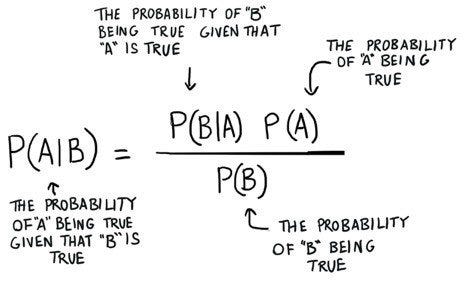
To look at dependent events, we often use the Bayes theorem, which is given by the formula below:
Ok, that’s very useful, but how do we know these probabilities? In basic exercises, usually we have probabilities that are easy to calculate, with things such as coins and dice. But how do we deal with more complicated probabilities? We work with cumulative distribution functions, which give us the probabilities of finding a value smaller (or greater) than another value we set. For example, if we knew the distribution of people’s heights in our town, we could calculate the probability of finding someone shorter (or taller) than 1.80m. From this function, we can derive the probability distribution, that gives us the probability that a value will fall within a certain range (we could know the probability of someone being between 1.70m and 1.80m tall, for example).
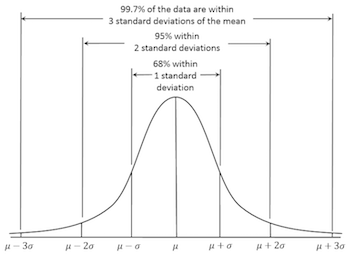
Some distributions are particularly important since they are often found in many real-life phenomena: Bernoulli, Binomial, Poisson and Gaussian, to mention a few. The Gaussian distribution is particularly important because of the Central Limit Theorem that states that, for any given distribution, when we sample the population many times, the means of those samples will follow a Gaussian distribution with the same mean as the original population.
Gaussian distribution. Source: Wikipedia
Probability distributions are a huge subject, and there’s a lot of content out there on it. It is out of the scope of the book to go into the details of each of them but it’s an interesting subject to study further.
Estimation and inference
Once we have our probability distribution, we want to be able to make estimations from a given sample. For example, let’s say we sample a few students in a school, get their ages and want to estimate the average age in the school. There are mainly two approaches to it: Maximum Likelihood and Least Squares. The first one reasons that our estimation of the average age in the population should be the one that makes the sampled result the most likely. The latter tries to find the estimation that will yield the smaller difference between estimated values and observations. And how do we choose an estimator? Ideally, we want an unbiased estimator, such that it is expected to give us a true result, but also one that doesn’t vary too much depending on the sample we take.
What if we want to estimate an interval, instead of a single point? It is also possible, due to something called confidence interval. A confidence interval can be calculated from the distribution we have, and will allow us to make a statement more or less like “I’m 95% confident that the average age in this school is between 10 and 12”, which can be quite useful for decision-making.
Another important statistical method is called hypothesis testing, which is used to test if your parameter takes a specific value or lies within a specific range. Let’s say we want to know if men and women earn the same. We sample a group of men and a group of women, calculate their average wages and find out that men earn in average $35,000 a year and women make $33,000. Ok, can we really say that those populations are essentially different? What if women earned $34,999, could we also reach the same conclusion? How big should this difference be so that we can say its statistically significant? We set a level of confidence we want to have (say 95%) and test our hypothesis. There are many ways of doing it, depending on what we are testing and on the population distribution but, if we do it right, our test will indicate us if our hypothesis holds or not.
Statistical models
A statistical model is some simple representation or description of the system we are studying. Since it is a simplification, we’ll necessarily lose information in this process, so we try not to lose the most important bits.
“All models are wrong, some models are useful” — George Box
Models can be mechanistic, based in a solid underlying theory (such as gravity) that allows us to predict some behaviour (an object falling, for example) or empirical, more common in the social sciences, where we try to infer the theory from observed data.
They can also be exploratory, where we try to find relationships and patterns (ex.: looking at demographic data to see if there are characteristics that are correlated) or confirmation models, where we test our conjectures to see if they are supported by data.
Finally, they can be split into descriptive models, where we try to characterise our data, calculating means, standard deviations, etc., or predictive models, were we try to infer some variable’s behaviour based on the other variables.
Predictive models are quite useful and they can be very simple or very complicated, usually depending on the number of explanatory variables we use. However, more complicated models do not always yield better predictions. Sometimes, adding more information makes models so specific for our sample that they do not generalise well for the whole population. This phenomenon is called overfitting.
Statistical models are often based on the idea of correlation: when two variables are correlated, it means that observing a value for one of them gives us a hint on the value of the other. For example, height and weight: tall people tend to be heavier and heavy people tend to be taller. Obviously, tall people can be light and heavy people can be short, but there’s still an overall trend. Correlation can also be negative, for example temperature and hot chocolate sales: the higher the temperature, the less people buy hot chocolate. Correlation is usually represented by a correlation coefficient that goes from -1 (perfect negative correlation) to 0 (no correlation at all) to 1 (perfect positive correlation). It is very important to keep in mind that correlation does not mean causation. For example, ice cream sales and deaths by drowning are correlated, but one does not cause the other, it’s just that in warmer days people buy more ice cream and swim more, so usually when ice cream sales go up it’s because it’s a warm day, meaning more people will swim (and drown).
In the end, the author briefly goes through some important statistical methods that are worth checking in more detail:
Regression analysis: it allows us to say “someone who weights 83kg is expected to be 1.83m tall”, based on a sample, even if we haven’t sampled anyone who’s 83kg. The most basic type of regression is linear regression, which supposes a linear relationship between two variables, as per the example below:
In the plot above, we can see our sample data (the dots) and the estimated regression line that will allow us to make estimations.
Analysis of variance (ANOVA): it allows us to compare means from many different populations and test if they are significantly different or not.
Clustering: used for finding groups of observations that are very similar. We just set the number of groups we want in the end and the algorithm gives us the best partitions.
Linear Discriminant Analysis (LDA): technique for finding the best linear combination of features in order to characterise different observations. Roughly, it helps us find attributes that are good at differentiating observations.
K-nearest neighbours (KNN): method used to estimate an attribute of a specific observation, based on the K observations that are the most similar to it.
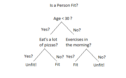
Decision tree: it is a very intuitive model used to estimate a certain characteristic (numeric or not) for a given variable, based on decision rules:
Time series: there is a whole domain in statistics dedicated to studying how certain variables fluctuate on time, based on concepts like trend and seasonality.
Factor analysis: in summary, it tries to find factors that are responsible for the shared variance between the observed variables.
Cross-validation: to avoid overfitting, we should not test our models on the same data they were trained on. There are many different methods that allow us to do that, such as splitting our sample data into two groups, one for training and one for testing.
Bootstrapping: it’s a good technique for getting better models, by sampling observations and replacing them within the actual sample.
Survival analysis: for example, imagine studying impacts of a disease in people’s lifetimes. After 20 years of study, some people have died, some haven’t. How do you deal with those who didn’t die, since you do not know their total lifetime yet? If you remove them from the study, you remove everyone who survived, and you will estimate a lifetime shorter than it actually is. Survival analysis deals with this sort of specificity.
Statistical computing
With the advent of computers, most of the calculations needed for statistical analysis can be done within seconds with softwares such as R, which really helped this field to grow, and made statistician’s work a lot easier and more productive. On the other hand, it made it easier to apply methods without mastering how they actually work, leading sometimes to wrong results.
Conclusion
The book really covers a broad range of subjects, so of course it is not possible to go too deep in any of them. However, it’s a very good introductory book, specially for those who come from a non-mathematical background. It is important, though, to pick some subjects that seem more relevant to you and study them in more depth. I’ll give it 7/10.