Tag: data-science

System Design for AI Engineers
A pragmatic approach for interviews

I’ve been studying system design on my own and I feel that, as data scientists and AI engineers, we don’t see it enough.

At the beginning I was a bit lost, didn’t know many of the terms used in the domain.

I watched many Youtube tutorials, and most of them go into a level of detail that can be overwhelming if you’re not a software engineer.

Yet, many AI engineering jobs these days have a system design step in the recruiting process.

So, I thought it’d be a good idea to give an overview of what I’ve learned so far, focused on AI engineering.

This tutorial will be focused on system design interviews, but of course it can also help you learn system design in general, for your job.

I’ll be using a framework from the book “System Design Interview”, which suggests the following script for the interview:
1. Clarifying questions
2. Propose high level design and get buy-in
3. Deep dive
4. Wrap-up: refine the design
I’ve adapted this framework to make it more linked to AI Engineering, as well as more pragmatic, by outlining what I consider to be the minimum output required in each step.

And, for this tutorial, I took a question that I’ve seen in interviews for an AI Engineer position:

“Build a system that takes uploaded .csv files with different schemas and harmonizes them.”

So, let’s design!

Clarifying questions

In this first step, you should ask some general questions, to have a better view of the context of the problem, and some more specific ones, to define the precise perimeter you’re working on.

More specifically, you should end this step with at least this info:
- context
- functional features
- non-functional features
- key numbers
Context

Ask things like:
- who will be using this?
- how will they be using it?
- where they will be using it (ex.: is it just one country, or worldwide)?
In our case, the system will be used in-company, to format multiple .csv files that come from different sources.

Their format and schema can always be different, so we need a robust and flexible solution that handles well this variability.

Those files will be uploaded by users, that don’t need the file right away: they just need it to be stored somewhere for later use by other systems.

It’s a small company, and they are all more or less in the same place.

Functional features

These are the things the product/service should be able to do.

In our example, there’s only one main functional feature: convert file.

But, we can also split that into 3 steps, which will help ups design our system later:
- upload file
- process file
- store file
In a more complex app, like YouTube, functional features could be:
- upload video
- view video
- search video
- etc.
Make sure the interviewer is onboard with these. In a real-life situation, you’d have things like authentification, account creation, etc.

Non-functional features

These are things that your system should consider, like: scalability, availability, latency, etc.

In practice, there’s a few ones that you should almost always consider:
- latency
- availability vs. consistency
Latency means: what’s an acceptable time for the user to get a response?

The availability vs. consistency tradeoff refers to the idea that in a distributed system, you can’t always guarantee both that data is immediately consistent across all nodes and that it’s always available when requested — especially during network failures.

Example: Imagine a banking app where a user transfers money from their savings to their checking account. If the system prioritizes consistency, it might temporarily block access while syncing all servers to ensure the balance is accurate everywhere. If it prioritizes availability, it might show the new balance immediately — even if some servers haven’t updated yet — risking temporary inconsistencies.

In some services, availability is more important. In others, consistency is more important.

Don’t look at this at the system level, but at the level of each functional feature.

Our use case is very simple, with only one functional feature, and the choice between consistency and availability will depend on the type of data and how it’s used, so check with the interviewer.

For the latency, let’s assume anything under 1 minute is acceptable.

Key numbers

This will help you calculate the amount of data that goes through your system, as well as the storage needs.

In our use case, some important figures could be:
- daily active users (ex.: 100)
- files per user (ex.: 1)
- average file size (ex.: 1 MB)
With these 3 numbers, you can already estimate the data volume:
- daily: 100 x 1 x 1 MB = 0.1 GB
- yearly: 0.1 GB x 365 = 36.5 GB
Those numbers will help us choose the best solutions for processing and storage.

For this example, let’s also assume there isn’t huge variance in the file size (there won’t be files over 10 MB).

Propose high-level design and get buy-in

With all this in hands, it’s time to start designing.

The minimal output here would be:
- core entities
- overall system design
- address functional requirements
A single server design is a reasonable starting point for most use cases.

So, start with a user, a server, services and databases.

In our example, we can start with only one service, so the whole setup would look like this:

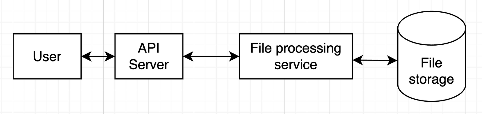
In a more complex system, we’d have more services and more databases.

Check with your interviewer if they’re OK with this and move on.

Deep dive

Now it’s time to detail the most important components of our previous design. That’s obviously the file processing service.

The minimal output:
- address non-functional requirements
But it’s also good to have these (check with the interviewer what they are expecting):
- API detail
- data schema detail
- tool choices
In our case, we should think in more detail on how those files would be processed.

My approach here (since we’re focused on AI solutions) is to use an LLM for this:
1. Give the LLM a “gold standard” format for our .csv files (column names and formats)
2. Give it a sample of the file to transform too (column names and formats)
3. Ask it for code that converts the file into the desired format
4. Run that code on the uploaded file
5. Store the resulting file
With this approach in mind, we can then look back into our design and what changes we should make to it:
1. We should probably separate code generation from code running, since these serve completely different purposes
2. There might be times when we get a file schema that we’ve seen already. In that case, we can have some sort of storage that allows us to cache code used before.
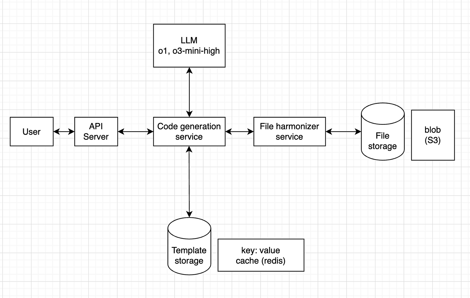
This would result in something like this:

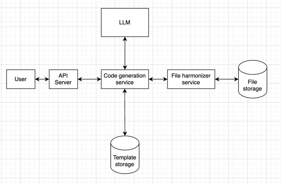
Meaning that the code generation service will first check in “template storage” if we have seen this format before.

If so, it will fetch the code from that storage and send it to the file harmonizer service.

If not, then it will call the LLM.

Now, one of the non-functional requirements was a latency under 1 minute.

Given the average file sizes, it’s reasonable to assume the whole thing will take less than 1 minute to run.

In terms of technical choices, a few things are relevant here:
- the type of model
- the type of storage
For the model, any model should do it, but I think it’s safer to go for a reasoning model, such as o1 or o3-mini-high.

For the file storage, since it’s just .csv files, a blob storage service like Amazon S3 should work.

For the template storage, we could have a key: value system, where the key is the schema (or a hash version of it) and the value is the corresponding code (or maybe a path to a blob storage with the .py file). One tool that can do this is Redis.

So, our final design would look like this:

Wrap up

In this step, we can refine our design, or at least find improvement opportunities.

Essentially, show what could be improved if you had more time.

In our case, here are some examples:
- a first iteration loop: what happens if the code fails to run? How do we call the LLM again, with the error message, to ask for new code?
- a fallback system: if the code fails n times in a row, how can we make sure it stops trying, and gives some error message to the user, instead of running an infinite loop?
- backup: how can we make sure our file storage has some sort of backup?
- simultaneous requests: how can we handle cases where multiple users upload at the same time? Should we use a message queue system?
The idea is to find bottlenecks, single points of failure and things like that, to improve on.

Conclusion and additional resources

I’ve seen many resources on system design interviews, and most of them are focused on software engineers, with very complex systems, addressing things that are usually not handled by AI engineers.

Yet, when the interview is for an AI engineer role, the request can often be more like this one: instead of multiple services and use cases, a sort of linear processing system, focused on LLMs, etc.

I’ve read two books on the topic:

“System Design Interview” is more generic, and I found it more useful, giving an overview of how to approach these interviews.

“Generative AI System Design Interview” is more focused on building things from scratch (LLMs, image generation models, etc.), which is not as common as using external APIs.

If you’re more into courses, I can recommend these two:
- Grokking the Modern System Design Interview
- Machine Learning System Design – AI-Powered Course
If you want a more detailed post on the topic, I found this one really useful:
- System Design For Beginners: Everything You Need in One Article
It goes straight to the point, with very practical advice.

And, if you prefer video format, I did one for this tutorial as well:

That’s it, I hope this was useful for you.

I’m not an expert in system design, and I’m aware that the design I propose above can be improved in many ways.

I just wanted to share what I’ve learned so far, focusing more on AI.

Let me know in the comments if you’d do anything different, or if you see any major flaws in that design.

Feel free to reach out to me if you would like to discuss further, it would be a pleasure (honestly):
- LinkedIn
- YouTube
13 April 2025
How to Fine-Tune an LLM with Hugging Face + LoRA
Fine-tuning is the process of taking a pre-trained model and adjusting it on a specific dataset to specialize it for a particular task.

Instead of training a model from scratch (which is costly and time-consuming), you leverage the general knowledge the model already has and teach it your domain-specific patterns.

It’s like giving a well-read intern a crash course in your company’s workflow — faster, cheaper, and surprisingly effective.

LoRA (Low-Rank Adaptation) is a clever trick that makes fine-tuning large models much more efficient.

Instead of updating the entire model (millions or billions of parameters), LoRA inserts a few small trainable matrices into the model and only updates those during training.

Think of it like attaching a lightweight lens to a heavy camera — you adjust the lens, not the whole system, to get the shot you want.

Under the hood, LoRA works by decomposing weight updates into two smaller matrices with a much lower rank (hence the name).

This dramatically reduces the number of parameters you need to train — without sacrificing performance.

It’s a powerful way to customize large models on modest hardware, and it’s part of why AI is becoming more accessible beyond big tech labs.

The dataset

For this tutorial, I’ve decided to use Paul Graham’s blog to build a dataset with his essays.

I really like his style of writing, and thought it’d be cool to have a fine-tuned model that mimics it.

To build the dataset, I scraped his blog, then reverse-engineered the prompts that could have been used to write his essays.

This means I gave each of his essays to ChatGPT and asked what prompt could have been used to generate it.

This resulted in a dataset containing a prompt and an essay, which we’ll use to fine-tune our model.

Now, let’s build!

Tutorial

Start by installing stuff:
```
!pip install bitsandbytes
!pip install peft
!pip install trl
!pip install tensorboardX
!pip install wandb
```
- bitsandbytes: efficient 8-bit optimizers for reducing memory usage during training
- peft: lightweight fine-tuning methods like LoRA for large language models
- trl: tools for training LLMs with reinforcement learning (e.g. PPO, DPO)
- tensorboardX: TensorBoard support for PyTorch logging and visualization
- wandb: experiment tracking and model monitoring with Weights & Biases
Next, let’s preprocess our data:
```
from enum import Enum
from functools import partial
import pandas as pd
import torch
import json

from transformers import AutoModelForCausalLM, AutoTokenizer, set_seed
from datasets import load_dataset
from trl import SFTConfig, SFTTrainer
from peft import LoraConfig, TaskType
import os

seed = 42
set_seed(seed)

# Put your HF Token here
os.environ['HF_TOKEN']="<your HF token here>" # the token should have write access

model_name = "google/gemma-3-1b-it"
dataset_name = "arthurmello/paul-graham-essays"
tokenizer = AutoTokenizer.from_pretrained(model_name)

tokenizer.chat_template = "{{ bos_token }}{% if messages[0]['role'] == 'system' %}{{ raise_exception('System role not supported') }}{% endif %}{% for message in messages %}{{ '<start_of_turn>' + message['role'] + '\n' + message['content'] | trim + '<end_of_turn><eos>\n' }}{% endfor %}{% if add_generation_prompt %}{{'<start_of_turn>model\n'}}{% endif %}"
def preprocess(sample):
    prompt = sample["prompt"]
    response = sample["response"]

    messages = [
        {"role": "user", "content": prompt},
        {"role": "assistant", "content": response}
    ]

    return {"text": tokenizer.apply_chat_template(messages, tokenize=False)}

dataset = load_dataset(dataset_name)
dataset = dataset.map(preprocess, remove_columns=["prompt", "response"])
dataset = dataset["train"].train_test_split(0.1)
```
Here, we set up the environment for fine-tuning a chat-style language model using LoRA and Google’s Gemma model.

We then format the answers to have a “text” field, containing both the prompts and the responses.

The result is a train/test split of the dataset, ready for supervised fine-tuning.

Now, we define our tokenizer:
```
model = AutoModelForCausalLM.from_pretrained(model_name,
                                             attn_implementation='eager',
                                             device_map="auto")
model.config.use_cache = False
model.to(torch.bfloat16)
```
Here, we:
- Load the model with attn_implementation='eager', which uses a more compatible (though sometimes slower) attention mechanism useful for certain hardware or debugging.
- Map the model to available devices (device_map="auto"), which automatically spreads the model across CPUs/GPUs as needed based on memory availability.
- Cast the model to bfloat16, a memory-efficient format that speeds up training/inference on supported hardware (like recent NVIDIA/TPU chips).
Next, we set up our LoRA parameters:
```
rank_dimension = 16
lora_alpha = 64
lora_dropout = 0.1

peft_config = LoraConfig(r=rank_dimension,
                         lora_alpha=lora_alpha,
                         lora_dropout=lora_dropout,
                         target_modules=[
                             "q_proj", "k_proj", "v_proj",
                             "o_proj", "gate_proj", "up_proj",
                             "down_proj"
                             ],
                         task_type=TaskType.CAUSAL_LM)
```
- r: rank dimension for LoRA update matrices (smaller = more compression)
- lora_alpha: scaling factor for LoRA layers (higher = stronger adaptation)
- lora_dropout: dropout probability for LoRA layers (helps prevent overfitting)
- target_modules : which layers we target. You don’t need to specify those individually, you can just set it to “all_linear”. However, it can be a good exercise to experiment with different layers (to check all the available layers, run print(model))
Next, we set up our training arguments:
```
username = "arthurmello" # replace with your Hugging Face username
output_dir = "gemma-3-1b-it-paul-graham"
per_device_train_batch_size = 1
per_device_eval_batch_size = 1
gradient_accumulation_steps = 4
learning_rate = 1e-4

num_train_epochs=10
warmup_ratio = 0.1
lr_scheduler_type = "cosine"
max_seq_length = 1500

training_arguments = SFTConfig(
    output_dir=output_dir,
    per_device_train_batch_size=per_device_train_batch_size,
    per_device_eval_batch_size=per_device_eval_batch_size,
    gradient_accumulation_steps=gradient_accumulation_steps,
    save_strategy="no",
    eval_strategy="epoch",
    logging_steps=logging_steps,
    learning_rate=learning_rate,
    max_grad_norm=max_grad_norm,
    weight_decay=0.1,
    warmup_ratio=warmup_ratio,
    lr_scheduler_type=lr_scheduler_type,
    report_to="tensorboard",
    bf16=True,
    hub_private_repo=False,
    push_to_hub=True,
    num_train_epochs=num_train_epochs,
    gradient_checkpointing=True,
    gradient_checkpointing_kwargs={"use_reentrant": False},
    packing=False,
    max_seq_length=max_seq_length,
)
```
Here, we set:
- per_device_train_batch_size and per_device_eval_batch_size set how many samples are processed per device at each step for training and evaluation, respectively.
- gradient_accumulation_steps allows effective batch sizes larger than memory limits by accumulating gradients over multiple steps.
- learning_rate sets the starting learning rate for model optimization.
- num_train_epochs defines how many times the model will see the full training dataset.
- warmup_ratio gradually increases the learning rate during the first part of training to help stabilize early learning.
- lr_scheduler_type="cosine" uses a cosine decay schedule to adjust the learning rate over time.
- max_seq_length defines the maximum number of tokens per training sequence.
Finally, we train our model:
```
trainer = SFTTrainer(
    model=model,
    args=training_arguments,
    train_dataset=dataset["train"],
    eval_dataset=dataset["test"],
    processing_class=tokenizer,
    peft_config=peft_config,
)

trainer.train()
```
Here, you should see something that looks like this:

This shows the training and validation loss for each epoch.

If training loss decreases and validation loss increases, this indicates overfitting (which we can see here around epoch 3).

Some strategies to adress overfitting include:
- reducing learning_rate
- increasing lora_dropout
- reducing num_train_epochs
Once you’re satisfied with the training results, you can compare your model’s output with the base model’s:
```
base_model = AutoModelForCausalLM.from_pretrained(model_name).to(torch.bfloat16)
base_tokenizer = AutoTokenizer.from_pretrained(model_name)

fine_tuned_model = model
fine_tuned_tokenizer = tokenizer

# Example input prompt
prompt = "<start_of_turn>user\Write an essay on the future of AI<end_of_turn><eos>\n<start_of_turn>model\n"

# Inference helper
def generate(model, tokenizer, prompt):
    device=model.device
    inputs = tokenizer(prompt, return_tensors="pt").to(device)
    output = model.generate(**inputs)
    return tokenizer.decode(output[0], skip_special_tokens=True)

print("=== Base Model Output ===")
print(generate(base_model, base_tokenizer, prompt))

print("\n=== Fine-Tuned Model Output ===")
print(generate(fine_tuned_model, fine_tuned_tokenizer, prompt))
```
There you go, now you have your own fine-tuned model to replicate Paul Graham’s style!

If you set push_to_hub=True in SFTConfig , you can call your fine-tuned model anytime, using your own username and output_id :
```
model = AutoModelForCausalLM.from_pretrained(
         "arthurmello/gemma-3-1b-it-paul-graham")
```
And, of course, you can adapt this approach to fine-tune LLMs for other use cases!

A video version of this tutorial is available here:

Feel free to reach out to me if you would like to discuss further, it would be a pleasure (honestly):
- LinkedIn
- YouTube
8 April 2025
Build a Neural Network From Scratch – in Less Than 5 minutes
No TensorFlow. No PyTorch. Just you, NumPy, and 20-ish lines of code.

We’re going straight to the core: how a neural network actually learns — and we’ll teach it the classic XOR problem.

The Problem: XOR

We want this network to learn the XOR rule:
```
0 XOR 0 = 0  
0 XOR 1 = 1  
1 XOR 0 = 1  
1 XOR 1 = 0
```
If A or B are equal to 1, then the output is equal to 1… unless they are both equal to 1, in which case the output is 0.

It’s a simple pattern… that isn’t linearly separable. A single-layer perceptron fails here. But with one hidden layer, it works.

Step 1: Setup and architecture

Let’s define our data and our tiny network.
```
import numpy as np

# XOR input and labels
X = np.array([[0,0],[0,1],[1,0],[1,1]])
y = np.array([[0],[1],[1],[0]])

# Define network architecture
input_size = 2
hidden_size = 4
output_size = 1
```
We’ve got:
- 2 input features (x1, x2)
- 4 neurons in the hidden layer
- 1 output (for binary classification)
Step 2: Initialize weights

Random weights, zero biases. Simple and effective.
```
np.random.seed(1)
W1 = np.random.randn(input_size, hidden_size)
b1 = np.zeros((1, hidden_size))
W2 = np.random.randn(hidden_size, output_size)
b2 = np.zeros((1, output_size))
```
We’ll learn these weights as we train.

Step 3: Activation functions

We’ll use sigmoid for both layers — good enough for this toy example.
```
def sigmoid(z): return 1 / (1 + np.exp(-z))
def sigmoid_deriv(a): return a * (1 - a)
```
sigmoid_deriv is the derivative — it tells us how much to adjust during backprop.

Step 4: Train it

Here’s the full training loop. Forward pass, backprop, and gradient descent.
```
learning_rate = 0.1
epochs = 1000

for epoch in range(epochs):
    # Forward pass
    A1 = sigmoid(X @ W1 + b1)      # hidden layer
    A2 = sigmoid(A1 @ W2 + b2)     # output layer

    # Backpropagation (compute gradients)
    dA2 = (A2 - y) * sigmoid_deriv(A2)
    dA1 = dA2 @ W2.T * sigmoid_deriv(A1)

    # Gradient descent (update weights and biases)
    W2 -= learning_rate * A1.T @ dA2
    b2 -= learning_rate * np.sum(dA2, axis=0, keepdims=True)
    W1 -= learning_rate * X.T @ dA1
    b1 -= learning_rate * np.sum(dA1, axis=0, keepdims=True)
```
This is the heart of every neural net:
- Forward pass: make a guess
- Backward pass: see how wrong you were
- Update: adjust weights to do better next time
Step 5: Make predictions

Let’s see if it learned XOR.
```
preds = sigmoid(sigmoid(X @ W1 + b1) @ W2 + b2) > 0.5

print("Predictions:\n", preds.astype(int))
```
Output:
```
[[0]
 [1]
 [1]
 [0]]
```
It works!

Where to go from here

You just built a functioning neural network from scratch.

Here’s what you can try next:
- Replace sigmoid with ReLU in the hidden layer
- Add a second hidden layer
- Swap out the loss function for cross-entropy
- Wrap this into a class and build your own mini framework
Final words

Learning how this stuff works under the hood is powerful.

You’ll never look at TensorFlow or PyTorch the same again.

No magic.
Just math.
Just code.

Here’s a video version of this tutorial:
31 March 2025
Why You’re Struggling to Break into Data Science
I see many people having a hard time transitioning from other fields into Data Science, even though there’s more open jobs every day. Many companies end up going for people who already have domain experience or who are fresh out of college, with a degree in Statistics or Computer Science.

Although it can be hard to make this transition, I did it, and I think you can do it too, as long as you have the right strategy.

Let’s take a look at some tips to help you land your first job.

Stop doing MOOCs

Don’t get me wrong, some online courses are great, but I feel that beginners tend to think that doing ten of those in a year will somehow help landing a job.

First, if you just do them for the sake of getting a certificate and putting it on LinkedIn, you won’t learn much. Plus, so many people have so many of those that most recruiters don’t care much about it.

Instead, do a few good ones at first, to have some understanding of the field and to be able to answer interview questions. The one I recommend is the famous Machine Learning specialization by DeepLearning.AI and Stanford, on Coursera. This will keep you busy and give you a good theoretical basis.

That next book will not help

The same logic goes for books: many people think that reading hundreds of books will make them magically absorb all that content and become machine learning experts.

Instead, use books as tools to gather specific knowledge that you need right now. Working on a Time Series project? Reading a book on the subject while you do it might help.

But again, don’t do it just to cross that item off your list, recruiters don’t care about how many books you read last year.

Choose the right side projects

Side projects help you in two ways: building skills and showing off your work. If your first project is doing logistic regression on the Titanic dataset, fine, you are warming up. But that’s not a great project for display.

Once you know the basics, try working on 2 or 3 projects that will actually display your skills to recruiters, such as deploying a model in production via a WebApp that you can show during an interview, creating a public dashboard or doing a deep analysis on some interesting dataset.

Some certifications help, others don’t

There are tons of certifications out there, so choose wisely. Usually, the hard ones also have the better payoffs: GCP, AWS, Azure and IBM certifications can be quite valuable. Tableau and Power BI too. The ones you get from just watching videos on Coursera, not so much.

If you are doing one of those I mentioned, check what are the most used cloud providers and dashboarding tools in your region, and focus on those.

Don’t be picky (at first)

If you are transitioning and haven’t been able to land a great job at first, don’t be picky. If you work in logistics and want to do Machine Learning, maybe a first job as a Data Analyst for a year will get you closer to your goal. Even if you are just doing Excel and dataviz, you are now closer than you were before, so look at it as a transitory move.

You might need to accept a lower salary at a not-so-great company too.

Choose a smooth transition

Let’s say you work in HR and want to transition to Data Science or Data Analysis. Focusing on data jobs related to HR analytics will make the transition smoother to you, and your set of skills will be valuable to your employer. They will be much more likely to accept your lack of data skills if you can make up for it with domain expertise.

Even if you don’t want to work with HR analytics forever, see this as a transitory move.

Start with consulting companies

There are many consulting companies out there who outsource data scientists and data analysts to other companies. They tend to pay less, but the bar might be lower, since they are currently hiring like crazy.

Do this for a couple of years and you will have enough experience to land a better paying job in the future.

Focus on your coding skills

Everyone will say during an interview how awesome they are, and how they have a unique skill set that differentiates them from competition.

Trust me, you are not the only one who knows how to “approach problems from a business perspective to get insights from data and generate actual value”.

Instead, build hard skills like Python and SQL, which will likely be tested during interviews, and can actually differentiate you from other candidates.

If you would like to discuss further, feel free to reach out to me on other platforms, it would be a pleasure (honestly):
- LinkedIn
- YouTube
23 March 2025
More Than Words: How AI Agents Are Changing Automation
Memory, reasoning, and the future of intelligent systems

AI is shifting from passive assistants to active problem solvers. Instead of just generating text based on a prompt, AI agents retrieve live information, use external tools, and execute actions.

Think of the difference between a search engine and a research assistant. One provides a list of links. The other finds, summarizes, and cross-checks relevant sources before presenting a well-formed answer. That’s what AI agents do.

Let’s break down how they work, why they matter, and how you can build one yourself.

Why AI Agents?

Traditional GenAI applications can generate convincing answers but lack:
- Tools: They can’t fetch real-time data or perform actions.
- Reasoning structure: They sometimes jump to conclusions without checking their work.
AI agents solve these issues by integrating tool usage, and structured reasoning.

Take a financial analyst, for example. Instead of manually searching for Apple’s stock performance, reading reports, and comparing it to recent IPOs, she could use an agent to:

1. Retrieve live stock data from an API.

2. Pull market news from a financial database.

3. Run calculations on trends and generate a summary.

No wasted clicks. No sifting through search results. Just a concise, actionable report.

How AI Agents Work

AI agents combine three essential components:

1. The model (Language understanding & reasoning)

This is the core AI system, typically based on an LLM like GPT-4, Gemini, or Llama. It handles natural language understanding, reasoning, and decision-making.

2. Tools (external data & action execution)

Unlike standalone models, agents don’t rely solely on their training data.

They use APIs, databases, and function calls to retrieve real-time information or perform actions.

Common tools include:
- Search engines for fetching up-to-date information.
- Financial APIs for stock prices, economic reports, or currency exchange rates.
- Weather APIs for real-time forecasts.
- Company databases for business insights.
3. The Orchestration Layer (Planning & Execution)

This is what makes an agent more than just a chatbot. The orchestration layer manages:
- Memory: Keeping track of previous interactions.
- Decision-making: Deciding when to retrieve information vs. generating a response.
- Multi-step execution: Breaking down complex tasks into logical steps.
It ensures that the agent follows structured reasoning instead of blindly generating an answer.

Thinking Before Acting: The ReAct Approach

One of the biggest improvements in AI agent design is ReAct (Reason + Act). Instead of immediately answering a question, the agent first:

1. Thinks through the problem, breaking it into smaller steps.

2. Calls a tool (if needed) to gather relevant information.

3. Refines its answer based on the retrieved data.

Without this structure, models can confidently hallucinate — generating incorrect information with complete certainty.

ReAct reduces that risk by enforcing a step-by-step thought process.

Example

Without ReAct:

Q: What’s the tallest building in Paris?

A: The Eiffel Tower.

(Sounds reasonable, but wrong. The Montparnasse Tower is taller if you exclude antennas.)

With ReAct:

Q: What’s the tallest building in Paris?

Agent:

1. “First, let me check the list of tall buildings in Paris.” (Calls search tool)

2. “The tallest building is Tour Montparnasse at 210 meters.” (Provides correct answer)

This approach ensures accuracy by retrieving data when necessary rather than relying on training data alone.

AI Agents in Action: Real-World Examples

Let’s explore some concrete applications with the smolagents framework, by HuggingFace.
```
from smolagents import CodeAgent, DuckDuckGoSearchTool, HfApiModel

model = HfApiModel()
agent = CodeAgent(tools=[DuckDuckGoSearchTool()], model=model)

query = "Compare Apple's stock performance this week to major tech IPOs."
response = agent.run(query)
print(response)
```
What happens here?

1. The agent searches for stock performance data using DuckDuckGo’s API.

2. It retrieves relevant comparisons between Apple and newly public companies.

3. If needed, it could summarize key financial trends.

Instead of giving a vague answer like “Apple’s stock is up”, the agent provides a structured comparison, making it more useful.

This example uses an existing search tool, but the smolagents framework allows you to build your own: it could be calling an API or writing in a database, sending an email.

Any Python function, really.

The Future of AI Agents

AI agents are shifting how we interact with AI.

Instead of just responding to prompts, they make decisions based on logic, and call external tools.

Where Are We Headed?

1. Multi-Agent Systems — Teams of specialized AI agents working together.

2. Self-Improving Agents — Agents that refine their own strategies based on past interactions.

3. Embedded AI — Assistants woven into workflows that anticipate problems before they arise.

AI isn’t just answering questions anymore — it’s solving problems.

Final Thoughts

The difference between an AI model and an AI agent is the difference between knowing and doing.

A model like ChatGPT is an information engine. It predicts words based on patterns.

An agent is an action engine. It retrieves data, runs calculations, and executes tasks.

This shift — from static responses to dynamic, tool-enabled intelligence — is where AI is headed.

The real challenge now isn’t just improving models, but designing intelligent, adaptive systems that can reason, act, and learn over time.

AI agents will augment human decision-making, making us faster, more informed, and better equipped to navigate an increasingly complex world.

And that’s a future worth paying attention to.

Sources
- Google’s whitepaper on agents
- The HuggingFace agents tutorial
- smolagents
- Some other random stuff I found online 🙂
17 February 2025
AI Is Not Taking Our Jobs
A quantitative exploration of the relationship between technology, labor and wealth

I see many people say AI will take our jobs any time now, based on the following narrative: the better AI becomes, the less companies will need us, therefore we will be replaced.

It’s an interesting chain of thought, but does it have the empirical basis to back it up? In other words, does reality match the story? Well, it doesn’t seem so.

It’s common to engage in this sort of discussion with well-thought arguments, based purely on conjectures, without looking at the existing body of scientific work nor at the data. I propose we take a tour of those two dimensions, to see if we can learn a thing or two from the empirical evidence.

Before we start, there is one link we need to establish: technology increases productivity. Here, we are talking from an economics perspective. Don’t think “when I have my cellphone I can’t work as much”. Here we are looking more at “the more technology in the world, the more we can produce with the same amount of work”.

This phenomenon is explained by the ability of technology to automate tasks, streamline processes, and facilitate the creation of new products and services. The intrinsic connection between technology and productivity is fundamental to understanding everything else you will read here.

With that out of the way, let’s see what science and data have to say about the impact of AI on our jobs.

Scientific work

Will AI take our jobs? This question can be seen as a specific case of the broader, more strucured question “does technology increase unemployment?”.

Unsurprisingly, this question has been asked by researchers many times before: a meta-analysis from 2022 that looked at 127 studies concluded that there is more evidence suggesting that technology creates net jobs than the other way around [1]. Their analysis specifically focuses on industrialized economies, to capture technological change at the frontier. They have also explored how this effect can be different depending on how we look at technology, but we will talk more about this later.

Some of the fear of AI comes from the narrative that, since AI makes us more productive, companies will need less of us to do the same job and, therefore, they will hire less of us. So, another study, from the European Central Bank [2], looked at the more general question “does productivity growth threaten employment?”. It turns out the answer is no. Even though some industries with higher productivity have seen fewer jobs, overall, the growth in productivity hasn’t really harmed employment. The study shows that one industry becoming more productive doesn’t automatically mean it will hire more people. However, it suggests that the positive impacts of productivity in one area can still create more jobs in other parts of the economy, offsetting any job losses in sectors with productivity gains. So, in the big picture, productivity growth has actually led to more jobs across various sectors. This study also concluded that current technology advances might bring a positive contribution to net jobs:

[…] the source of productivity growth matters for its aggregate employment consequences. Given that service sector productivity growth appears to have relatively strong employment spillovers, our findings suggest that the productivity growth spurred by the spread of (ultimately) general-purpose technologies such as robotics from heavy industry and into services may prove a boon for employment growth.

Anothery interesting study, from the OECD [3], spanning 13 countries over two decades, investigates the relationship between productivity, employment, and wages. It found a positive correlation between productivity growth and increased employment and wages, both at the firm and aggregate levels:

At the more aggregate level, the role of reallocation and links across industries becomes more evident. Yet also here, results confirm that productivity growth is, overall, associated with positive changes in employment and wages. Increasing employment among expanding firms tends to outweigh decreasing employment in shrinking or exiting firms. Furthermore, productivity gains at the industry level contribute to stronger employment growth in downstream industries through value chains.

Looking at AI more specifically, a panel study from 2023 shows evidence that it decreases the level of unemployment, at least in high-tech developed countries [4]. The study investigated how AI affects unemployment in 24 high-tech developed countries from 2005 to 2021, using Google Trend Index data related to AI and unemployment rates.

Data

Now, for some extra context, let’s take the time to explore some of the data ourselves, to answer some broeader questions. If technology is evolving (and I don’t think anyone questions that), and this is not decreasing the number of jobs available, then what is it doing for us?

We are not necessarily “less employed”

To contribute to the body of evidence that we are not being replaced by technology, let us look at the employment rates in the world since 1950:

Image by author

I put China and India separately because their data was not available for every year and, given their populations, this had a big impact on the variability of the indicator, specially since the 1990s.

We can see that, despite the impressive technological advances over the last 70 years, employment rates do not seem to be a bigger issue now than they were back then.

We are working less

We are, on the other hand, working much less than our ancestors:

Image by author

This global trend, however, is not the same everywhere:

Image by author

Richer countries are reducing their working hours at higher rate than the rest. I cherry-picked some specific countries that are representative of different trends:
- Germany is an example of a rich country where people worked much more than the rest of the world, and has drastically decreased since then;
- The US has become substantially richer since the 1950’s, yet its work load have not decreased significantly;
- China and India seem to be going in the opposite direction of the rest of the world, working longer hours.
We are richer than ever

I hope this does not come as a surprise, but we have never been richer:

Image by author

So, even though the world is working less, pretty much every country got richer.

Of course, the distribution of that wealth was not the same across the globe. Pretty much every country got richer, but some got richer than others (again, no surprise):

Image by author

But how can we work less and make more money? What allowed that to happen? Well, we happen to have become more productive over time thanks, in part, to technology.

We are more productive

Technology, education and solid institutions contribute to productivity, and we can see the results over the years:

Image by author

Unfortunately, I couldn’t find data older from before the 2000s but, given the decrease in number of hours worked and the increase in GDP per capita, we can see the trend is there and is pretty much strong.

This constant productivity increase over the time is what allows us to work less and make more money.

Things will still change

So, everything will stay the same? Well, no. Of course AI will have an impact in the job market. But the change might be more related to jobs migrating from one industry to another, and from one region to another.

The European Central Bank study [2] suggests that increases in productivity move jobs in two main ways:
1. less manufacturing jobs, more services jobs
2. less low-skill jobs, more high-skill jobs
More specifically, we expect more jobs in health, education, and services, and less jobs in utilities, mining, and construction.

Also, in the meta-analysis we saw earlier [1], they identify five key categories of technology measures in the literature, with different impacts on job markets:
1. Information and communication technology: more high-skill, non-routine, and service jobs;
2. Robots: the negative impact on employment is generally offset by new jobs related to their production, operation, and maintenance;
3. Innovation: product innovation seems to create jobs, but the evidence for process innovation remains mixed;
4. Productivity: job gains were mostly favorable for non-production, high-skill, and service jobs. Nonetheless, the net employment effects observed in these studies are rather negative than positive;
5. Other: other/indirect measures of technology indicate net job creation effects, particularly for non-production labour, but also for lowly skilled workers, particularly in service jobs.
So we could expect either:
1. relocation of jobs from manufacturing countries towards service-intensive countries;
2. a change in the sectorial structure within countries, with an increase of service jobs when compared to manufacturing;
3. a mix of both.
I imagine these changes could increase inequality due to:
1. the migration towards high-skill jobs, particularly if education doesn’t keep up;
2. more money going to capital owners: there is already evidence [2] that the share of labor on national income is decreasing.
We could be wrong, but how?

Of course this whole analysis could be wrong. Let’s try and gather some evidence that goes in the opposite direction, or at least understand in what ways the evidence we saw before could be inadequate.

There are some theoretical attempts to model the Marxist thesis of “labor immiseration”, looking at different axes:
1. Inter-generational market failure: quick advancements in technology benefit skilled workers and those who own capital in the short term. However, over time, it leads to hardships for people who cannot invest in physical or human capital;
2. Task encroachment: two opposing economic forces shape how much income goes to labor: technology advancement which replaces ‘old’ tasks, decreasing labor’s share of output, potentially lowering real wages; and internal technological progress that creates new tasks requiring labor. The interaction of these forces may result in a unbalanced growth path;
3. New tasks might not be created “fast enough”: the number of automated tasks could grow at a higher rate than the new tasks created by automation, leading to a reduction in the number of tasks that can be performed by humans;
These models are theoretical, though: they are not evidence that the net job losses will happen, they just outline scenarios where it could.

There is some evidence showing that this time could be different, and that this relationship between productivity and unemployment might be shifting: recent decades have witnessed more negative own-sector effects of productivity growth, especially in manufacturing, and less positive external effects on other-sector employment, possibly due to increased trade openness. However, this pattern has been seen before, in the 1980s, and it’s not new [2].

Another study, by the National Bureau of Economic Research [5], looks at the impact of increased industrial robot usage in the United States from 1990 to 2007 on local labor markets. The researchers find that the rise in robot usage leads to a significant negative effect on employment and wages across commuting zones. They support their findings by showing that areas most exposed to robots post-1990 did not display different trends before that period. The impact of robots is distinct from other factors like imports from China, decline of routine jobs, offshoring, and various types of IT capital. The conclusion suggests that for every additional robot per thousand workers, the employment to population ratio decreases by about 0.18–0.34 percentage points, and wages decrease by 0.25–0.5 percent. The study focuses specifically on industrial robots in certain local labor markets, which can’t account for the spillover effects on other regions or markets.

Maybe this time it’s different, and AI is such a disruptive technology that it will behave in a different way. Maybe, its relationship with productivity is different than other technologies.

Maybe. But the empirical evidence suggests otherwise, so I wouldn’t bet on it.

References
11 February 2025
How to Become an AI Expert in 5 minutes
Impress colleagues and dazzle recruiters without actually knowing anything about AI

Forget years of research, hands-on coding, or grueling math — this guide will teach you everything you need to fake it until you make it in the world of AI.
1. Say “garbage in, garbage out.” It means nothing, but it sounds cool.
2. Ask what LLM they’re using. It’s absolutely irrelevant, but it makes you sound like you know what you’re talking about. Bonus points if you tilt your head and say, “Oh, GPT-4? Interesting choice.”
3. Talk about “the black box problem.” You don’t need to know what it actually means — just sigh heavily and say, “That’s the thing with AI, isn’t it? It’s all a black box.” Everyone will nod solemnly.
4. Use “fine-tuning” in every other sentence. You don’t need to understand the difference between fine-tuning and prompt engineering. Just say things like, “Well, it’s not performing well because they probably didn’t fine-tune it properly.”
5. Mention ethical concerns vaguely. Say, “We need to consider ethical issues here too.” But never specify which ethical problems you’re referring to. If pressed, just shake your head and mutter: “Bias, man. It’s everywhere.”
6. Throw in words like “unstructured data” and “scalability.” For example: “The issue is that most companies can’t handle unstructured data at scale.” People will assume you’re deep into AI architecture, even if you’re just deep into Twitter.
7. Make wild predictions about AI taking over. Alternate between saying, “AI will replace 80% of jobs in the next five years,” and, “AI is overhyped; it’ll never truly replace humans.” Contradict yourself freely — it’s all part of the mystique.
8. End every conversation with “We’re still in the early days of AI.” It’s the perfect way to sound both optimistic and profound while giving yourself an exit strategy.
Congratulations! You are now ready to dazzle coworkers and intimidate LinkedIn connections with your newfound AI “expertise.”

Just remember: when in doubt, say “It’s all about the data.” No one will argue.
11 February 2025
Book Summary: Statistics — A Very Short Introduction

How can we apply statistical methods to real-world problems?

Who should read this book?

You either work with data or want to start to, but come from a tech background or just don’t remember much from Stats 101, and need a refresh on the basics of statistics.

One-paragraph summary

It’s a good starting point to understanding statistics: it approaches a broad range of topics, from basic probability to random forests, without going too deep in any of them, so no previous mathematical background is required.

Full summary

Introduction

The author starts by giving a series of possible definitions for statistics, one of them being “the technology of extracting meaning from data”.

“Statistics is hocupocus with numbers” — Audrey Habera and Richard Runyon

He then gives a glance of the many different applications that are possible with statistics, from public policy to marketing to spam filtering, and mentions some of the issues that can arise from misusing it. The most notable example is the Sally Clark case: in 1999, a young British lawyer was sentenced for life for killing her two baby children who she claimed had died from cot death. The sentence was based on the testimony of Sir Roy Meadow, the prosecution’s paediatrician, that said that it was nearly impossible that this was the actual cause, since the chances of this happening to two children was of 1 in 73 million. The verdict was then that the mother was guilty. The probability calculated by the doctor was, however, flawed: he did it by multiplying the probability of one cot death two times. This method, however, needs the two events to be independent, which they are not, considering that, given that one of the children died from it might indicate genetic conditions that will also manifest in the second child.

This, and many other examples, show that statistics has an important role in society: providing evidence. Without it, we cannot subject our opinions to test, and they remain mere speculations.

Statistics began on the end of the 19th century only as discursive explorations of data. In the first half of the 20th century it evolved and became a more mathematics-oriented field. Only in the second half of the 20th century it faced its latest revolution with the use of computers, which allowed the field to develop its methods and apply heavy-computational algorithms.

Descriptions

In statistics, we analyse objects and their attributes usually in the shape of observations and variables. This information can, sometimes, be overwhelming, so we might want to aggregate it by doing simple summary statistics: average, dispersion, skewness and quantiles, for example.

The concept of average can comprise many formal concepts, but the most used case is the arithmetical mean: the sum of all values, divided by the number of observations. For example, if we wanted to understand the attribute “age” for a given classroom of college students, instead of looking at all the students’ ages, we sum them all, divide by the number of students, and get 22 years. It doesn’t mean all students are 22 years old, but it gives us an overall picture: some are older, some are younger, but we can imagine it is not a classroom full of kids, for example.

However, let’s take a second example: there’s five people, four of them earn $5,000 a month and one of them earns $100,000 a month. In average, these people make $24,000 a month. However, this does not fully describe their real situation, since it is not a group of people where everyone earns more or less $24,000. From here we can add the concept of dispersion: how far from the average are the values in this group? One measure of dispersion is the variance, calculated by taking the square of the difference between all the numbers and the mean, and then calculating their averages. Wouldn’t it be simpler to just take the mean without the square part? Yes, but then positive and negative values would reduce each other’s effects, cancelling out the whole purpose of measuring dispersion. We can take the square root ofthe variance as another measure, called the standard deviation.

Ok, so we know the average and whether the dispersion is high or low, but how exactly is the shape of this dispersion? For this, we can look at skewness and quantiles. Skewness measures the lack of symmetry in the population: if it’s very asymmetric, there are many more values higher or lower than the average. Quantiles tell you what value you should take if you want a certain percentage of the population below this value, and there are a few types of quantiles. One of the most common is the percentile: if you are in the 90th percentile of your classroom’s grades, it means you have better grades than 90% of the your classroom.

Collecting good data

“Garbage in, garbage out” — Everyone data science article out there

When collecting data for analysis, it is very important to pay attention to its quality: no matter how sophisticated are your models, if you put bad data in, your outcome will also be poor.

Pay special attention to missing data: sometimes it’s random but sometimes it can also reveal an underlying pattern. For example, when asking people for their income, people who get really good (or really bad) salaries may prefer not to answer, generating missing data that can actually give you some information. To deal with missing data, you can ignore it, remove those observations/variables or you can try to input it by replacing them by something simple such as the sample mean or by something a lot more complex, using prediction algorithms. It will depend mostly on your data and your goals. When data is incorrect, on the other hand, most of the time there’s not much that can be done a posteriori so avoid making these mistakes when fetching data.

When it comes to data sources, they can basically be of two types: observational or experimental. The first one comes from real-life observations whereas the latter comes from controlled experiments. Experimental studies are better for isolating variables and causation effects but they are usually harder to do. When conducting experiments, we should plan very well our experiment design: choosing the best groups for measuring the impact of each variable, taking into account the effect of interactions. For example, if we want to test the effect of a new drug, we should have a control group and a test group, sampled randomly from the population, ideally with similar characteristics. If the test group has only men and the control group has only women, we won’t be able to know if the observed results were the effect of the drug or of the subject’s gender.

For this kind of procedure, we can apply techniques from a statistics domain called survey sampling, which can help us the best methods of sampling individuals within a population.

Probability

Another definition of statistics is “the science of handling uncertainty”, which is what the study of probability tries to address. A lot of its utility is based on the Law of Large Numbers, which roughly means that, if when you toss of a coin you have 50% chances of getting heads, then the more you throw the coin, the closer the overall proportion of heads will be to 50%.

This leads us to the two main approaches when it comes to probability: frequentist and Bayesian. Roughly, frequentists see probabilities as the proportion of times the event would occur if the exact same circumstances were repeated infinitely. The Bayesian approach takes into account the amount of information available: probability is subject to how much we know, and thus it changes as we gather new information.

Whatever approach you take, you will encounter the idea of independence between events. Basically, two events being independent means that the occurrence of one of them does not affect the probability of the other one occurring. If we throw two coins separately, the fact that we got heads in one does not change the probability of getting heads in the second one.

To look at dependent events, we often use the Bayes theorem, which is given by the formula below:

Skymind’s beginner’s guide to the Bayes theorem

Ok, that’s very useful, but how do we know these probabilities? In basic exercises, usually we have probabilities that are easy to calculate, with things such as coins and dice. But how do we deal with more complicated probabilities? We work with cumulative distribution functions, which give us the probabilities of finding a value smaller (or greater) than another value we set. For example, if we knew the distribution of people’s heights in our town, we could calculate the probability of finding someone shorter (or taller) than 1.80m. From this function, we can derive the probability distribution, that gives us the probability that a value will fall within a certain range (we could know the probability of someone being between 1.70m and 1.80m tall, for example).

Some distributions are particularly important since they are often found in many real-life phenomena: Bernoulli, Binomial, Poisson and Gaussian, to mention a few. The Gaussian distribution is particularly important because of the Central Limit Theorem that states that, for any given distribution, when we sample the population many times, the means of those samples will follow a Gaussian distribution with the same mean as the original population.

Gaussian distribution. Source: Wikipedia

Probability distributions are a huge subject, and there’s a lot of content out there on it. It is out of the scope of the book to go into the details of each of them but it’s an interesting subject to study further.

Estimation and inference

Once we have our probability distribution, we want to be able to make estimations from a given sample. For example, let’s say we sample a few students in a school, get their ages and want to estimate the average age in the school. There are mainly two approaches to it: Maximum Likelihood and Least Squares. The first one reasons that our estimation of the average age in the population should be the one that makes the sampled result the most likely. The latter tries to find the estimation that will yield the smaller difference between estimated values and observations. And how do we choose an estimator? Ideally, we want an unbiased estimator, such that it is expected to give us a true result, but also one that doesn’t vary too much depending on the sample we take.

What if we want to estimate an interval, instead of a single point? It is also possible, due to something called confidence interval. A confidence interval can be calculated from the distribution we have, and will allow us to make a statement more or less like “I’m 95% confident that the average age in this school is between 10 and 12”, which can be quite useful for decision-making.

Another important statistical method is called hypothesis testing, which is used to test if your parameter takes a specific value or lies within a specific range. Let’s say we want to know if men and women earn the same. We sample a group of men and a group of women, calculate their average wages and find out that men earn in average $35,000 a year and women make $33,000. Ok, can we really say that those populations are essentially different? What if women earned $34,999, could we also reach the same conclusion? How big should this difference be so that we can say its statistically significant? We set a level of confidence we want to have (say 95%) and test our hypothesis. There are many ways of doing it, depending on what we are testing and on the population distribution but, if we do it right, our test will indicate us if our hypothesis holds or not.

Statistical models

A statistical model is some simple representation or description of the system we are studying. Since it is a simplification, we’ll necessarily lose information in this process, so we try not to lose the most important bits.

“All models are wrong, some models are useful” — George Box

Models can be mechanistic, based in a solid underlying theory (such as gravity) that allows us to predict some behaviour (an object falling, for example) or empirical, more common in the social sciences, where we try to infer the theory from observed data.

They can also be exploratory, where we try to find relationships and patterns (ex.: looking at demographic data to see if there are characteristics that are correlated) or confirmation models, where we test our conjectures to see if they are supported by data.

Finally, they can be split into descriptive models, where we try to characterise our data, calculating means, standard deviations, etc., or predictive models, were we try to infer some variable’s behaviour based on the other variables.

Predictive models are quite useful and they can be very simple or very complicated, usually depending on the number of explanatory variables we use. However, more complicated models do not always yield better predictions. Sometimes, adding more information makes models so specific for our sample that they do not generalise well for the whole population. This phenomenon is called overfitting.

Statistical models are often based on the idea of correlation: when two variables are correlated, it means that observing a value for one of them gives us a hint on the value of the other. For example, height and weight: tall people tend to be heavier and heavy people tend to be taller. Obviously, tall people can be light and heavy people can be short, but there’s still an overall trend. Correlation can also be negative, for example temperature and hot chocolate sales: the higher the temperature, the less people buy hot chocolate. Correlation is usually represented by a correlation coefficient that goes from -1 (perfect negative correlation) to 0 (no correlation at all) to 1 (perfect positive correlation). It is very important to keep in mind that correlation does not mean causation. For example, ice cream sales and deaths by drowning are correlated, but one does not cause the other, it’s just that in warmer days people buy more ice cream and swim more, so usually when ice cream sales go up it’s because it’s a warm day, meaning more people will swim (and drown).

In the end, the author briefly goes through some important statistical methods that are worth checking in more detail:

Regression analysis: it allows us to say “someone who weights 83kg is expected to be 1.83m tall”, based on a sample, even if we haven’t sampled anyone who’s 83kg. The most basic type of regression is linear regression, which supposes a linear relationship between two variables, as per the example below:

Trying to predict muscle strength based on lean body mass. Taken from http://www.jerrydallal.com

In the plot above, we can see our sample data (the dots) and the estimated regression line that will allow us to make estimations.

Analysis of variance (ANOVA): it allows us to compare means from many different populations and test if they are significantly different or not.

Clustering: used for finding groups of observations that are very similar. We just set the number of groups we want in the end and the algorithm gives us the best partitions.

Linear Discriminant Analysis (LDA): technique for finding the best linear combination of features in order to characterise different observations. Roughly, it helps us find attributes that are good at differentiating observations.

K-nearest neighbours (KNN): method used to estimate an attribute of a specific observation, based on the K observations that are the most similar to it.

Decision tree: it is a very intuitive model used to estimate a certain characteristic (numeric or not) for a given variable, based on decision rules:

Simple decision tree taken from this article: https://bit.ly/2vwM2fp

Time series: there is a whole domain in statistics dedicated to studying how certain variables fluctuate on time, based on concepts like trend and seasonality.

Factor analysis: in summary, it tries to find factors that are responsible for the shared variance between the observed variables.

Cross-validation: to avoid overfitting, we should not test our models on the same data they were trained on. There are many different methods that allow us to do that, such as splitting our sample data into two groups, one for training and one for testing.

Bootstrapping: it’s a good technique for getting better models, by sampling observations and replacing them within the actual sample.

Survival analysis: for example, imagine studying impacts of a disease in people’s lifetimes. After 20 years of study, some people have died, some haven’t. How do you deal with those who didn’t die, since you do not know their total lifetime yet? If you remove them from the study, you remove everyone who survived, and you will estimate a lifetime shorter than it actually is. Survival analysis deals with this sort of specificity.

Statistical computing

With the advent of computers, most of the calculations needed for statistical analysis can be done within seconds with softwares such as R, which really helped this field to grow, and made statistician’s work a lot easier and more productive. On the other hand, it made it easier to apply methods without mastering how they actually work, leading sometimes to wrong results.

Conclusion

The book really covers a broad range of subjects, so of course it is not possible to go too deep in any of them. However, it’s a very good introductory book, specially for those who come from a non-mathematical background. It is important, though, to pick some subjects that seem more relevant to you and study them in more depth. I’ll give it 7/10.

2 February 2025
Book Summary: Agile Data Science 2.0

Building full-stack data analytics applications with Spark

Who should read this book?

You are already a Python experienced user, with some knowledge in Spark, and you want to fill your knowledge gaps while building a full data science application from scratch with a front-end interface.

One-paragraph summary

The book is a step-by-step guide on how to build an application for analytics, including downloadable scripts. It will give you an initial overview of the Agile method, and how to apply it to data science, but 80–90% of the book will be hands-on tutorials. In the end, you should have built an HTML page that estimates delays for a given flight, gathering data from different sources.

Full summary

This book is basically a big tutorial, and since there is no point summarising a tutorial, the summary will focus only on the more general parts that talk about agile and data science.

“Agile Data Science is an approach to data science around web application development” — The book

In addition to what the above quote says, the author starts the book by defining Agile Data Science as “a methodology for analytics products development, mixing the best software development practices, but adapting them to the iterative nature of data science”.

The Agile Data Science Manifesto

One of the key steps towards Agile Data Science is constantly shipping intermediate output: no matter if something is still a draft or you are not sure the data is correct, ship it to your internal user for validation. This will avoid wasting time on features people do not need, and will also help you spot issues early on. This also means documenting the whole thinking process and not just the final product.

That kind of process will also help reducing technical debt, defined as “a concept in programming that reflects the extra work that arises from building code that is easy to implement in the short run, instead of using the best overall solution”.

Since data science development is a very iterative process, it is impossible to determine deadlines beforehand. Instead, agree beforehand with you stakeholders that you cannot give them a precise final date, but that will you ship constant progress reports. These reports do not have to be actual formal reports, but a front-end interface that shows the current shape of your data, which will also help you get constant feedback.

People management

“In Agile, we value generalists over specialists” — Also the book

In a standard data science project, there can be several roles, one for each step of the process. In Agile, we try to make the team leaner, by getting generalists instead of specialists. In general, this means we want someone to be a business developer, marketer, and product manager at the same time, someone else can be the experience designer, interaction designer, and web developer, then a third person can take over the roles of an engineer, data scientist, and researcher, and finally someone to be both a platform engineer and a DevOps Engineer. This means 4 people doing the job of 11. Although there are less people involved, there is a lot of synergy between these functions, so we compensate in productivity.

For this setup to work, it is better to use third-party high-level tools and platforms, instead of developing everything in-house. It will save you a lot of overhead time, so you can focus on what really matters.

If you manage a data science team, focus more on overseeing all the experiments that are happening simultaneously throughout the team, than in handing tasks for each one.

Finally, make sure your developers share their code with each other for peer-review, or code together. This will help finding errors and making code more readable for future users.

Agile tools

The typical data flow comprises at least 5 different types of tools, used in a sequential order.

Collectors: the tools used to collect and log events (events are the occurrences we want to measure, such as clicks and purchases). Ex.: Kafka

Bulk storage: filesystem capable of parallel access by many concurrent proceses. Ex.: Amazon S3 and Hadoop (companies are more and more using Amazon S3 instead of Hadoop).

Distributed document stores: multi-node stores using a document format. Ex.: MongoDB

Application server: it plumbs JSON files from the distributed document store through to the client, allowing for visualisation. Ex.: Python/Flask, Ruby/Sinatra, Node.js.

Browser/application: it displays data visualisation and possibly interactive tools. It can be a dedicated app or an ordinary internet browser, to display HTML pages.

The Data-Value Pyramid

The Data-Value Pyramid shows all the added-value we can get from data in a shape that highlights the importance of foundations: you cannot optimally get value from your reports, for instance, if you have not yet worked properly on plumbing your records and displaying basic charts. This is valid from a project perspective, but also from a company’s point of view: companies should have solid foundation on how their records are collected, and sound understanding of basic charts before moving on to building reports or trying to implement recommendation systems. This process allows for constant iteration in each step before moving on to the next. The project built in the book is based on these steps, with the author detailing each of them with examples:

Records

These are the foundation of your pyramid: make sure you are collecting exactly the events you want and make many tests to check for inconsistencies. Then, display those records in a front-end interface and exchange with your stakeholders. This will help you see if you are working with the right data and avoid wasting time in the future.

Charts

Charts are the first and simplest way to have proper visual representation of your data. You probably won’t be able to get your charts right at first, so try different approaches and iterate with the feedback you get. In the end, make sure your chart tells a story.

Reports

Reports are a set of charts or tables and other additional information, eventually with interactive features. Make sure you know the kind of information your end users need by exchanging information, and understand how they interact with your report, so you can choose the interactive features. They can be built from the charts you already have.

Predictions

“Prediction is very difficult, especially if it’s about the future” — Nils Bohr, Nobel laureate in Physics

Here is where the value of data starts showing: seeing what happened in the past is good, but being able to predict the future is great. The example used in the book is a model that tries to predict flight delays based on time of departure, airport and even aircraft information. There are essentially two types of prediction models out there: regression and classification. Roughly speaking, regression deals with problems where you will have a quantitative output in the end, such as predicting a house price or someone’s weight, whereas classification deals with categorical outputs: predicting someone’s football team or social class.

Actions

Finally, this is the most important part: information is only worth something if you can act on it. The book does not describe this step, but it could have been a good idea to give some examples of direct action originated by data science. Instead, it ends by improving its predictive model. It is very important to know what actions you will take based on your prediction data, ideally before calculating it. This helps you avoid “vanity metrics”: metrics you look at to feel good but don’t help you make any decisions.

Conclusion

Since all the code comes with the book, it is very easy to just sit back and follow the script, which won’t help you a lot. Instead, try to not only run the scripts but to understand them and, eventually, change and adapt them for your personal use cases. Without the coding part, there is actually not much content left in the book, so the name can be a bit deceiving: you get this very specific tutorial without much explanation on Agile and/or Data Science. It is a good book to have around in case you need some ideas for a data application setup, but nothing you cannot find online with a bit of effort. I’d give it a 6/10.

P.S. Make sure you have 16GB of RAM or are willing to pay for a virtual machine in AWS, otherwise you will not be able to follow through.

2 February 2025

References

1. Somers, M., Theodorakopoulos, A., & Hötte, K. (2022). “The fear of technology-driven unemployment and its empirical base.”
2. Autor, D., & Salomons, A. (2017, June 19). “Does Productivity Growth Threaten Employment?”
3. Calligaris, S., Calvino, F., Reinhard, M., & Verlhac, R. (OECD). (2023). “Is there a trade-off between productivity and employment? A cross-country micro-to-macro study.” OECD Science, Technology and Industry Policy Papers, №157.
4. Guliyev, H. (2023). “Artificial intelligence and unemployment in high-tech developed countries: New insights from dynamic panel data model.” Economic Research Center of Turkish World, Azerbaijan State Economic University.
5. Acemoglu, Daron and Pascual Restrepo. (2017). “Robots and Jobs: Evidence from U.S. Labor Markets.” NBER Working Paper №23285, March.