
Have you ever felt like there’s a strange trade-off in the people you date — the kinder they are, the less attractive they seem? Or maybe doctors notice that patients either have diabetes or high blood pressure, but rarely both?
That’s Berkson’s Paradox in action. It’s a statistical illusion that happens when we only look at a filtered or biased sample. The relationships we see inside that sample can be completely different (even reversed) from what’s true in the broader population.
The Hospital Example
Imagine a hospital that only admits patients who have either:
- a high diabetes score, or
- a high blood pressure score.
In the general population, those two health issues are positively correlated: people with one often have the other.
But in the hospital’s dataset, something strange happens: if a patient doesn’t have high diabetes, they’re likely admitted because of high blood pressure, and vice versa.
This makes the two look negatively correlated, even though they’re not.
Let’s illustrate that with code.
cov = [[1, 0.4], [0.4, 1]]

# Generate data
diabetes_bp = np.random.multivariate_normal(mean, cov, n)
diabetes, bp = diabetes_bp[:, 0], diabetes_bp[:, 1]

# Define admission rule
admitted = (diabetes > 1.2) | (bp > 1.5)

# Create the DataFrame
df = pd.DataFrame({
    'Diabetes': diabetes,
    'BloodPressure': bp,
    'Admitted': admitted
})

# Plot
plt.figure(figsize=(6, 6))
plt.scatter(df[~df['Admitted']]['Diabetes'], df[~df['Admitted']]['BloodPressure'],
            color='pink', label='Not Admitted', alpha=0.6)
plt.scatter(df[df['Admitted']]['Diabetes'], df[df['Admitted']]['BloodPressure'],
            color='blue', label='Admitted', alpha=0.7)

# Threshold lines for admission
plt.axvline(x=1.2, color='gray', linestyle='--')
plt.axhline(y=1.5, color='gray', linestyle='--')

plt.xlabel("Diabetes Score")
plt.ylabel("Blood Pressure Score")
plt.title("Berkson's Paradox: Biased Hospital Admission (Weaker True Correlation)")
plt.legend()
plt.grid(True)
plt.tight_layout()
plt.show()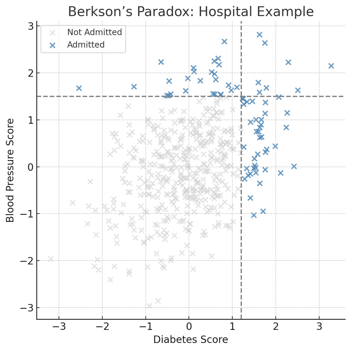
What You’ll See
In the full population, there’s a mild positive correlation: as diabetes goes up, so does blood pressure.
But when you only look at admitted patients, the correlation flips. It looks like people with high diabetes are less likey to have high blood pressure, and vice versa.
That’s Berkson’s Paradox. When you filter your data (whether it’s based on admissions, hiring decisions, or dating preferences ) you might create patterns that don’t exist in reality.
Why It Happens
Berkson’s Paradox is a result of conditioning on a collider: a variable that is influenced by two other variables. In this case:
Diabetes → Admission ← Blood Pressure
When we only look at patients who were admitted (filtering on the collider), it introduces a spurious negative correlation between diabetes and blood pressure, even if they are independent or positively correlated in the full population.
This is a known pitfall in causal inference, especially when working with observational data.
When It Matters
Berkson’s Paradox isn’t just academic. It can creep into real-world decisions:
- Healthcare: Hospitals analyzing only admitted patients might draw false conclusions about disease relationships.
- Dating apps: If you only swipe on people who are either attractive or kind, you may think those traits never come together.
- Hiring: Companies screening only the top of the resume pile might think strong technical skills and good communication never overlap.
- Product feedback: Analyzing only users who contact support may show misleading patterns about product problems.
In each case, you’re filtering the data in a way that distorts the truth.
Real-World Origin
Berkson’s Paradox was first described in a 1946 paper by Joseph Berkson, a statistician at the Mayo Clinic.
He noticed that certain diseases seemed negatively correlated in hospital data, even though there was no such relationship in the broader population.
You can find the original paper here:
Berkson, J. (1946) — Limitations of the Application of Fourfold Table Analysis to Hospital Data
It’s one of the earliest documented examples of how selection bias can warp statistical conclusions.
Key Takeaway
Be careful with filtered data. If you’re only seeing a slice of the population, the relationships in your data might be misleading. Berkson’s Paradox is a good reminder that how you collect your data can shape what you think it says.

